Hello IntervalLinearAlgebra.jl
Hello everyone and welcome to the first blog of my GSOC'21 project. Here I will give a short project overview and present the first results I have obtained so far.
Project overview
The purpose of the project is to develop IntervalLinearAlgebra.jl a package to perform numerical linear algebra rigorously, i.e. using interval arithmetic. The package is fully written in Julia and is built on top of IntervalArithmetic.jl for interval computations.
Basic concepts
As we are working with interval arithmetic, the most fundamental mathematical structure is interval. An interval \([a, b]\) is defined as a subset of \(\mathbb{R}\) as follows
\[ [a, b] = \{x \in \mathbb{R} | a \le x \le b \} \]Next, we introduce the concept of interval matrix, that is a matrix whose entries are intervals. More formally, let us denote by \(\mathbb{I}\mathbb{R}\) the set of real intervals. Then an interval matrix \(\mathbf{A}\in\mathbb{I}\mathbb{R}^{m\times n}\) is defined as
\[ \mathbf{A} = \{ A \in \mathbb{R}^{m\times n} | A_{ij} \in \mathbf{A}_{ij}, 1\le i \le m, 1\le j \le n\} \]Hence an interval matrix can be thought as a set of real matrices. Let us give an example
\[ \mathbf{A} = \begin{bmatrix} [2, 4]&[-2,1]\\ [-1, 2]&[2, 4] \end{bmatrix} \]is an interval matrix and for example
\[ A_1=\begin{bmatrix} 2&0\\ 1.5&3 \end{bmatrix} \in \mathbf{A} \]but
\[ A_2=\begin{bmatrix} 2&0\\ 1.5&8 \end{bmatrix} \notin \mathbf{A} \]Interval linear systems
At the moment, the functionalities of the package are limited to solve square interval systems, that is systems in the form
\[ \mathbf{A}\mathbf{x}=\mathbf{b} \]where \(\mathbf{A}\in\mathbb{I}\mathbb{R}^{n\times n}\) and \(\mathbf{b}\in\mathbb{I}\mathbb{R}^n\).
Now it's legitimate to ask the question: what does it mean to solve an interval linear system, in other words, what is \(\mathbf{x}\)? It is defined as
\[ \mathbf{x} = \{x \in \mathbb{R}^n | Ax=b \text{ for some } A\in\mathbf{A}, b\in\mathbf{b} \} \]in other words \(\mathbf{x}\) is the set of solutions of the real linear systems \(Ax=b\) for which \( A\in\mathbf{A}\) and \(b\in\mathbf{b}\). Again, the interval linear system can be thought as a set of real linear systems. The solution of the interval linear system is the set of solutions of the real linear systems in the interval system.
Characterizing the solution of an interval linear system
We now know what an interval linear system is and what solving it means. But how do we solve it? A naive approach would be to use Montecarlo, i.e. to randomly sample elements from the intervals and solve the several random real systems. Hopefully, repeating several times, we will get a good approximation of the true solution. Let us try it. Suppose we want to solve the linear system
\[ \begin{bmatrix} [2, 4]&[-2,1]\\ [-1, 2]&[2, 4] \end{bmatrix}\mathbf{x} = \begin{bmatrix} [-2, 2]\\ [-2, 2] \end{bmatrix} \]first let us import IntervalArithmetic.jl to define the matrix and vector. Since we are planning to solve several thousands of instances of the interval problem and we are working with small arrays, we can use StaticArrays.jl to speed up the computations.
using IntervalArithmetic, StaticArrays

A = @SMatrix [2..4 -2..1; -1..2 2..4]
b = @SVector [-2..2, -2..2]
2-element StaticArrays.SVector{2, Interval{Float64}} with indices SOneTo(2)
:
[-2, 2]
[-2, 2]To perform Montecarlo, we need to sample from the intervals. This can be achieved using the rand function, for example
rand(1..2)1.6291348873684761we are now ready for our montecarlo simulation, let us solve \(100000\) random instances
N = 100000

xs = [rand.(A)\rand.(b) for _ in 1:N]
100000-element Vector{StaticArrays.SVector{2, Float64}}:
[-0.44889606428857604, 0.3928096488422731]
[0.7961509062448051, 0.21261565245738948]
[-0.21652683334642917, -0.14026594625705752]
[0.2780614734829664, -0.08300975077387636]
[-0.09553601785839375, -0.9070371038176132]
[0.4054651040742707, 0.40021765448010016]
[-0.8137129912700739, -0.177550318111634]
[0.2822411518015633, 0.250135048167971]
[-0.15235580069558002, 0.2310472175067912]
[-0.23406607169530733, 0.5566371448674734]
⋮
[0.19690305714223466, -0.16718205313829992]
[0.03447064311292888, -0.6304584802868007]
[0.18876670332677647, 0.19224372028424622]
[0.4736864339328689, 0.08625234706181056]
[-0.17587467167618367, 0.5901451469686299]
[0.1383723642923509, 0.6101938606469426]
[0.187315914769036, 0.045985125281754205]
[0.2638363596614852, -0.22754940002799534]
[-0.5025052110421537, -0.28679114075137596]and let's plot the solution
using Plots

x = [xs[i][1] for i in 1:N]
y = [xs[i][2] for i in 1:N]

scatter(x, y, leg=false, ratio=1, alpha=0.5)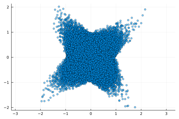
Looks a little messy, let us plot 2D-histogram instead
histogram2d(x, y, ratio=1)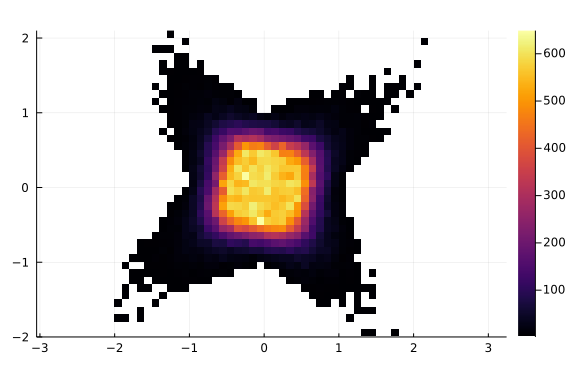
as we can see, most of the solutions seem to be condensed close to the origin, but repeating the experiments enough times we also got some solutions farther away, obtaining a star looking area. Now the question is, do we have the whole star?
Before we answer the question, we need to recall a couple of concepts from interval arithmetic. Given an interval \(X = [a, b]\), we define:
the center \(mid(X) = \frac{a+b}{2}\)
the radius \(rad(X) = \frac{b-a}{2}\)
let us also denote
the center matrix \(A_c = mid(A)\)
the radius matrix \(A_\Delta = rad(A)\)
where the operations mid and rad are applied to the matrices elementwise.
We are now ready to state the Oettli-Präger theorem, which says that an interval linear system \(\mathbf{A}\mathbf{x}=\mathbf{b}\) is equivalent to the set of real inequalities
\[ |A_cx-b_c| \le A_\Delta|x| + b_\Delta, \]where the absolute values are to be taken elementwise.
We have now transformed the set of interval equalities into a set of real inequalities. How to find the set of points satisfying those inequalities? IntervalConstraintProgramming.jl comes to the rescue!
So to solve the interval linear system we should
write the inequalities using Oettli-Präger
solving the inequalities using
IntervalConstraintProgramming.jl
IntevalLinearAlgebra.jl has a function that does all of this for you! Let's import it, note we also need to import IntervalConstraintProgramming.jl
using IntervalLinearAlgebra, IntervalConstraintProgrammingthen we need an initial enclosure of the solution. We will discuss later how to find this, for now, let us just cheat and rabbit out a good initial guess
X = IntervalBox(-5..5, 2)[-5, 5]²at the moment, we also need to provide a list of variables, this will be automated soon!
vars = (:x, :y)(:x, :y)now we can solve the interval linear system using Oettli-Präger theorem
p = oettli(A, b, X, vars)Paving:
- tolerance ϵ = 0.01
- inner approx. of length 13712
- boundary approx. of length 7489to understand what p is we would need to go into the specifics of IntervalConstraintProgramming.jl. Let's just say that p has two lists of small interval boxes, one containing those boxes strictly inside the solution set and one containing the boxes at the boundary.
Finally let us plot the solution on the same figure with the 2d-histogram
plot(p.inner, legend=false, ratio=1, lw=0)
plot!(p.boundary)
histogram2d!(x, y)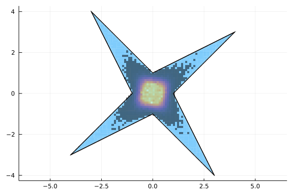
as we can see, the original montecarlo approximation, despite the high number of iterations, was pretty disappointing.
Conclusions
We have discussed what an interval linear system is and observed that it solution set can have a complex non-convex shape. We also gave a theorem that can be used to characterize the solution of the interval linear system. However, there are a couple of open issues
how do we find the starting enclosure?
Oettli-Präger becomes unpractical in higher dimensions
both points can be summarized into one
how can we find a tight interval box (a vector of intervals) containing the solution of the interval linear system?
The answer of this question will be the topic of the next blog entry. Stay tuned!